Continuous Probability Distributions
Continuous Random Variables
A continuous random variable is a function from a continuous sample space to a continuous set of numbers. Continuous random variables are measured values, like length, time, weight.
For example, let the random variable X measure the lengths of a certain species of tropical fish. The sample space and values of X obviously cannot be listed in a table as for a discrete random variable.
Probability Distribution of a Continuous Random Variable
The probability distribution of a continuous random variable comes from increasing the number of classes in a probability histogram. This is a histogram where the heights of the rectangles represent probabilities.
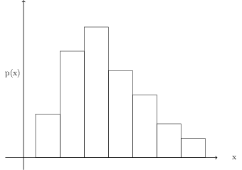
We would like to have the areas of the rectangles represent probabilities, that is, instead of \[ \begin{align} \sum p_i &= 1 \end{align} \ \] we would like \[ \begin{align} \sum f(p_i)\Delta x &= 1 \end{align} \ \] where f(pi) is some function of the probabilites and \( \Delta x \) is the width of the class rectangles.
If the number of classes in the histogram increases
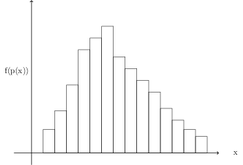
then each pi will approximate a point on a smooth curve and pi will become p(xi), which means f(pi) will become f(xi) and the expression for the sum becomes \[ \begin{align} \sum f(x_i)\Delta x &= 1 \end{align} \ \]
As the number of class rectangles increases indefinitely, the sum will more and more closely approximate an integral \[ \begin{align} \sum f(x_i)\Delta x \quad -> \quad \int f(x)dx \end{align} \ \] The function f(x) which determines the set of possible values of the random variable is called a probability density function (pdf) or simply, a probability distribution.
Note - the above discussion is not a proof but is included by way of motivation.
Probability and Continuous Probability Distributions
The properties of a continuous probability density function f(x) should have similar properties to those of a discrete distribution.
Corresponding to the property that the probabilities are non-negative and sum to one, we have \[ \begin{align} f(x) &\ge 0 \\ \int_{-\infty}^{\infty} f(x)dx &= 1 \\ \end{align} \ \] Note that because functions are defined over the real line, the integration limits must be \( \pm \infty \) to account for all possible values of x.
There are two possibilities when evaluating these types of integrals - in the first case, many pdfs are defined only for a finite interval. In this case
Example If a pdf is defined as \[ \begin{align} f(x) &= 2x \quad \text{ for } (0 \le x \le 1) \\ &= 0 \quad \text{elsewhere} \\ \end{align} \ \] then the interval becomes a finite interval and \[ \begin{align} \int_{-\infty}^{\infty} f(x)dx &= \int_0^1 2xdx \\ &= \left [ \frac{2x^2}{2} \right ]_0^1 \\ &= 1 \end{align} \ \]
 If a pdf is defined as
\[ \begin{align}
f(x) &= 3e^{-3x} \quad \text{for } x \ge 0 \\
&= 0 \quad \text{elsewhere}
\end{align} \ \]
Evaluate \(\int_{-\infty}^{\infty} f(x)dx\).
If a pdf is defined as
\[ \begin{align}
f(x) &= 3e^{-3x} \quad \text{for } x \ge 0 \\
&= 0 \quad \text{elsewhere}
\end{align} \ \]
Evaluate \(\int_{-\infty}^{\infty} f(x)dx\).
In the second case, you can handle an infinite limit by replacing it with a finite limit and let the finite limit increase without bound.
Example If a pdf is defined as \[ \begin{align} f(x) &= 2e^{-2x} \quad \text{ for } (x \ge 0) \\ &= 0 \quad \text{elsewhere} \end{align} \ \] then \[ \begin{align} \int_{-\infty}^{\infty}f(x) dx &= \int_0^{\infty} 2e^{-2x} dx \\ &= [ -e^{-2x}]_0^N \\ &= -e^{-2N} - (-e^0) \\ &= 1 \end{align} \ \] as N increases without bound.
Guided Examples
O E Qs
Here are two more properties of continuous pdfs
(1) The probability of X taking a value in the interval (x1, x2) is \[ P(x1 \lt X \lt x2) = \int_{x1}^{x2} f(x)dx \]
(2) The probability of the random variable X assuming a particular value is 0, i.e. \[ \begin{align} P(X=a) &= P(a \lt x \lt a) \quad \\ &= \int_a^a f(x)dx \\ &= 0 \quad \end{align} \ \] because of the properties of the definite integral.
Cumulative Distribution
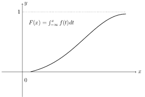
The cumulative distribution of a probability density function f(x), is denoted by F(x) and is defined as: \[ \begin{align} F(x) = P(X \lt x) &= \int_{-\infty}^x f(t)dt \end{align} \ \] which means the density function f(x) is \[ \begin{align} f(x) &= \frac{d}{dx} F(x) \end{align} \ \]
If a pdf is defined as
\[ \begin{align}
f(t) &= 3e^{-3x} \quad \text{for } x \ge 0 \\
&= 0 \quad \text{elsewhere}
\end{align} \ \]
find F(x).
To compute the probability that a score falls within a certain interval \[ \begin{align} P(a \lt X \lt b) &= \int_{a}^{b} f(x)dx \\ &= F(b) - F(a) \\ \end{align} \ \]
Example If \[ \begin{align} f(x) &= \frac{1}{2}e^{-x/2} \quad \text{ for } x \ge 0 \\ &= 0 \quad \text{ elsewhere } \end{align} \ \] then Pr(X < 4) is \[ \begin{align} \text{Pr}(X \lt 4) &= \int_0^4 \frac{1}{2}e^{-t/2} dt \\ &= [ -e^{-t/2}]_0^4 \\ &= -e^{-4/2} - (-e^0) \\ &= 1 - e^{-2} \end{align} \ \]
The graph of a cumulative distribution has the same behaviour as a cumulative histogram:
Conditional Probability
You can calculate the conditional probabilities of a continuous probability density functions using the rules for conditional probability.
If (a < b < c) is an interval, and X is a random variable, then \[ \begin{align} \text{Pr}(a \lt X \lt b | X \lt c) &= \frac{\text{Pr}(X \lt b \cap X \lt c)}{\text{Pr}(X \lt c)} \\ &= \frac{\text{Pr}(X \lt b)}{\text{Pr}(X \lt c)} \end{align} \ \] because in this case, the intersection of the two intervals is equal to the shortest.
Example If \[ \begin{align} f(x) &= \frac{1}{2}e^{-x/2} \quad \text{ for } x \ge 0 \\ &= 0 \quad \text{ elsewhere } \end{align} \ \] then \[ \begin{align} \text{Pr}(0 \lt X \lt 3 | X \lt 4) &= \frac{\text{Pr}(X \lt 3)}{\text{Pr}(X \lt 4)} \end{align} \ \] and Pr(X < 3) is \[ \begin{align} \text{Pr}(X \lt 3) &= \int_0^3 \frac{1}{2}e^{-x/2} dx \\ &= [ -e^{-x/2}]_0^3 \\ &= -e^{-3/2} - (-e^0) \\ &= 1 - e^{-3/2} \end{align} \ \] so \[ \begin{align} \text{Pr}(0 \lt X \lt 3 | X \lt 4) &= \frac{1 - e^{-3/2}}{1 - e^{-2}} \end{align} \ \] using Pr(X < 4) from the previous example.